MDI Interpolated Intensitygrams

We developed this 96-minute interpolated flattened intensitygram data series, mdi.fd_Ic_interp, for classifying regions (like sunspots) in paired (magnetogram,photogram) images. (For the context of that work, go up here).
This note describes this data series and how it is computed in case the series is useful to others doing studies on the joint data set.

Overview

We use the MDI 96-minute cadence line-of-sight (LOS) magnetograms (mdi.fd_M_96m_lev182) as the primary source of information for the classification of photospheric activity types. But, the MDI 6-hour cadence pseudo-continuum photograms (mdi.fd_Ic_flat) are also helpful, e.g., to distinguish faculae from weak sunspots. To use both images at the same time, we must temporally interpolate a photogram to the magnetogram time and disk parameters. This interpolated flattened photogram is then used with a LOS magnetogram to find sunspots and faculae. The approach we now use is similar to one used in earlier classification work (Turmon, Pap, and Mukhtar, Astrophys. Jour., 568(1), 2000; hereafter TPM2000), but improved in several ways in the light of this experience.

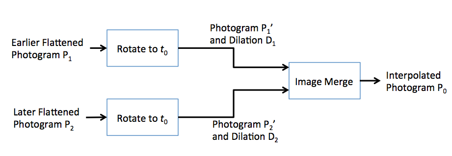
The basic approach is to find a bracketing pair of photograms for each magnetogram time, to rotate them into the desired coordinate frame, and finally merge the pair of rotated images:

In the diagram, the magnetogram sets the desired coordinate frame and observation time t₀. The bracketing photograms P₁ and P₂ are at times t₁ and t₂ (t₁ ≤ t₀ ≤ t₂), with separate, known, coordinate frames. The quantities marked "dilation" in the diagram are measures of image quality that we discuss below, along with the rest of the process.

Those uninterested in details about process can skip to the conclusion for usage notes. Browse products showing these images are nearby.

Finding Bracketing Photograms

The magnetograms control the observation times needed, but for computational reasons, a list of "good" photograms (eligible for inclusion in brackets) is found once, and used for all needed interpolations. To be considered "good", the photogram QUALITY must be non-negative (i.e., its most significant bit must be zero), and all necessary metadata must be present (some photogram records have good QUALITY, but their WCS are incomplete). Also, we enforce that the photogram is not in a list of about 130 known-bad photograms. These seem acceptable based on QUALITY and WCS, but are nevertheless unusable, e.g. some contain pervasive image artifacts or erroneous-but-present WCS. The excluded images are thus unusable for almost any purpose.

Then, for each magnetogram record, the tightest pair of bracketing photograms is found. Tightness is measured by comparing T_OBS values, which record actual observation time and can differ significantly from the nominal T_REC. Some brackets are too wide to use. The temporal width of the bracket is measured by a gap criterion

W = time-to-closer + 0.4 * time-to-farther,

where time-to-closer is the lesser of the two gaps

abs(T_OBS₀ - T_OBS₁), abs(T_OBS₀ - T_OBS₂),

and time-to-farther is the greater of the two. The reason for the unequal weighting is that after the images are merged, the closer image plays a much stronger role in the final photogram than does the farther one (see below).

The gap criterion W is recorded as IIXTCRIT (in seconds) in the metadata. If W is larger than 18 hours, we set a warning bit in QUALITY; if larger than 36 hours, we set a different bit in QUALITY, which indicates interpolation failed. In our experience, interpolation across larger gaps than 36 hours yields questionable results, even for large regions, due to morphology changes.

When W > 36 hours, even though interpolation fails, we still produce a data segment (by setting the entire interpolated image to the nominal quiet-sun value 1). Producing a segment may seem like a surprising design choice, but this made our downstream processing more uniform.

Because of the presence of such gaps due to failed interpolation, to use the interpolated intensity images, you MUST check QUALITY for these values:

0x10000 => W > 18 hours [probably still OK]
0x20000 => W > 36 hours: all-quiet placeholder segment [not OK to use]
0x40000 => used trivial interpolation for any reason

Checking QUALITY & 0x40000 (262144 decimal) will be sufficient for most
purposes. (For this data series, there is no distinction between bit 0x20000 and 0x40000.)

Note that, whenever the high bit in the magnetogram QUALITY is set, indicating missing data, a matching or "placeholder" record is created in the interpolated photograms, also with the high bit of QUALITY set. Of course, there is no segment in such records, but this ensures that there is a 1:1 relationship between magnetogram records and interpolated photogram records. This relationship simplifies logic when iterating over (magnetogram, photogram) pairs.

Rotating Photograms

After the bracket is found, both the earlier (t₁) and later (t₂) photograms are rotated into the new coordinate frame at t₀. This is done separately for each image by iterating over each pixel in the t₀ frame and projecting it back into the source image pixel array. It will typically have fractional values and therefore land between four pixels in the source image. Bilinear interpolation is used to approximate a value.

Standard formulas (Zappala & Zuccarello, Astron. Astrophys.(242), 1991; hereafter ZZ1991) for the latitude-dependent angular velocity of active regions in the photosphere,

Ω = 14.643 - 2.2407 sin²(lat) deg/day

are used to handle the time difference. This is a star-centered or sidereal rate; we account for observer motion by using the CRLN_OBS keywords.

Sunspot age, which we do not account for, changes Ω above by about 0.3 deg/day (ZZ1991, p. 483). Different observation and measurement techniques change the deduced values of Ω reported by several authors by a similar amount (J. G. Beck, Sol. Phys.(191), 2000, Fig. 3). A 9-hour rotation to find a nearby image (needed by less than 7% of the MDI photograms we labeled) corresponds to a movement of about 36 MDI pixels at disk center. An error in Ω of 0.3 deg/day over 9 hours corresponds to a displacement of about one pixel at disk center, a minor error. However, it is evident that as the interpolation interval stretches to 18 or 36 hours, the error due to this source is not always minor. This effect, combined with morphology changes over similar time scales, are the fundamental limiting factors on this method.

Combining Two Photograms

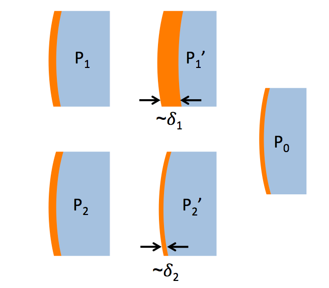
The two photograms contain duplicate information: estimates about t₀ using the past (P₁') and the future (P₂'). We would like to combine them in a way that properly weights their uncertainty, which comes from both spatial dilation and temporal decorrelation.

Consider dilation. P₁' is less accurate around the east limb because of foreshortening; a few values at the east limb of the original image P₁ may be stretched over many times more pixels in the rotated image P₁', with a corresponding distortion or smoothing of region boundaries. On the other hand, at the west limb, pixels in the same image P₁ will be compressed spatially in forming P₁'. Note that this compression does not, in the end, provide a resolution increase relative to (say) disk center, because the final resolution is a fixed value and the extra interstitial pixels are in effect thrown away.

One way to capture this is by a dilation map D, which is computed at the same time as the rotation &emdash; smaller is better.

D(i, j) = max{1, area[dest(i, j)] / area[source(i, j)]}

where area[dest(i, j)] is the solid-angle area of the (i, j) pixel in the destination frame, and area[source(i, j)] is that in the source frame. Clipping the result from below at one accounts for the fact, noted above, that resolution increase is not possible. In practice, the pixel areas are computed using the slope of the tangent plane at the pixel center, and the ratio is also capped at a high value (10⁴) to avoid infinities.

Here is a pair of discrepancy maps, D₁ on the left and D₂ on the right.
The colormap scale runs from 1 to 2.

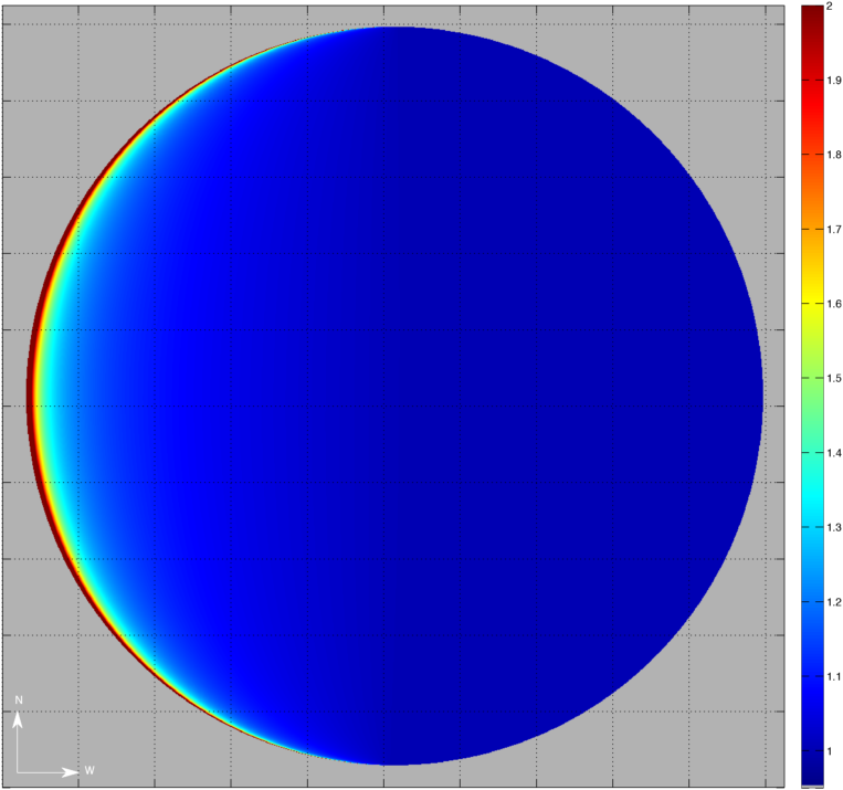
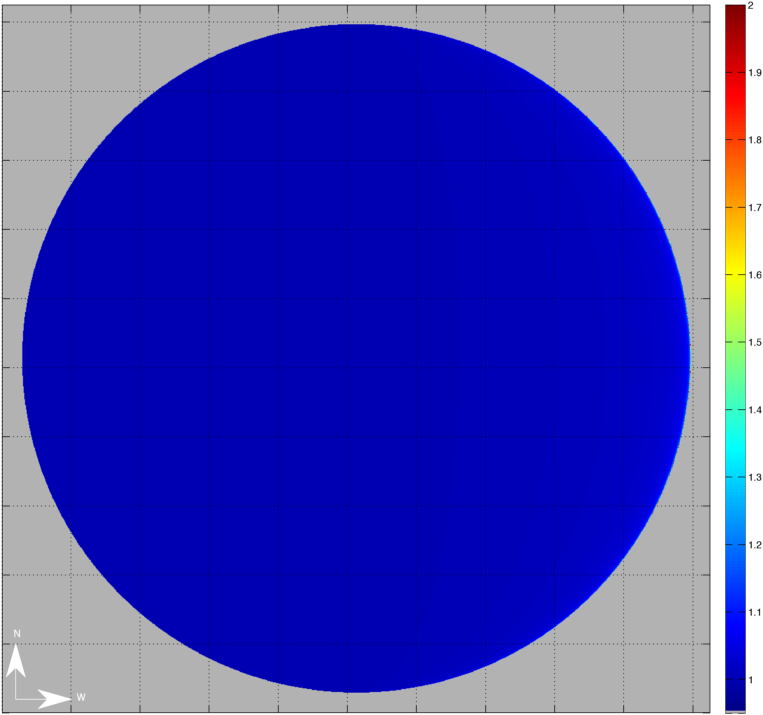
The prior image, rotated forward by 10 hours, shows a noticeable peak in discrepancy at the limb, while the later one, rotated backward by about 1 hour, does not. The plot below shows a section through disk center (row 512 of 1024), running from east to west, with D₁ in blue and D₂ in red. In this case, we wish to account for the increased uncertainty of the prior image, relative to the later image, at the east limb.

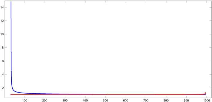
Dilation is important at the limb. On the other hand, the accuracy of the rotated images around disk center, where the dilation is near-unity, depends mainly on the (nonnegative) time gaps:

δ₁ = T_OBS₀ − T_OBS₁

δ₂ = T_OBS₂ − T_OBS₀

We combine these sources of information by computing, for each pixel (i, j),

Δ₁(i, j) = δ₁ D₁(i, j)

Δ₂(i, j) = δ₂ D₂(i, j)

These Δ values are taken to be proportional to the variances of random variables that are centered about the desired value P₀(i, j). The appropriate averaging in this case has weights proportional to the variance ratio, and summing to unity, i.e.

w(i, j) = Δ₂(i, j) ⁄ [ Δ₁(i, j) + Δ₂(i, j) ]

and then

P₀(i, j)= w(i, j) P₁(i, j) + [1 − w(i, j)] P₂(i, j)

This is the best linear unbiased estimate of P₀.

Of course, if one or the other rotated value is missing at (i, j), it is ignored in the result and the non-missing value is used as-is. If both are missing (see below), then the result is also recorded as missing.

Behavior at the Limb

In the source data series of flattened MDI intensitygrams, the last two to three pixels are reported as not-a-number. These narrow strips of unknown values fatten or shrink after rotation, and thus typically appear near the limb of the rotated intensitygrams P₁' and P₂'.

The image-merge process combines these two images, and the narrow unknown strips in one image are mostly filled in by valid values in the other one. But there are frequently a few hundred pixels where the unknown strips in P₁' and P₂' happen to overlap, and a not-a-number is reported in P₀. The precise fill-in pattern depends on the way the strips overlap, which in turn depends on the time gaps.

The disposition of a few pixels at the extreme limb is not very important in itself, but note that the width of the not-a-number strip depends on the time gaps. When examining browse movies of the interpolated images, the effect is that one can notice a faint pulsation (with a period controlled by the gap between flattened intensitygrams, nominally six hours) as these strips grow to about one pixel wide in a few places, and then shrink to nothing. The eye-catching pulsation seems to signal a problem with geometry, but it is not.

For definiteness, the situation is shown schematically below. Not-a-number pixels are in orange, known values in blue, and the east limb is detailed. To begin with, both source photograms have unknown strips of similar widths. The width of the unknown strip in P₁' increases as δ₁ grows. On the other hand, that for P₂' is largest when δ₂ is zero, because P₂' is being pushed eastward as δ₂ grows, squeezing the strip of unknowns. The final width in P₀ is the smaller of the two. So as time advances, δ₂ decreases toward zero, and the width increases; eventually, the reference "later" image jumps forward, δ₂ rises suddenly, and the width of the strip drops (typically) to zero.

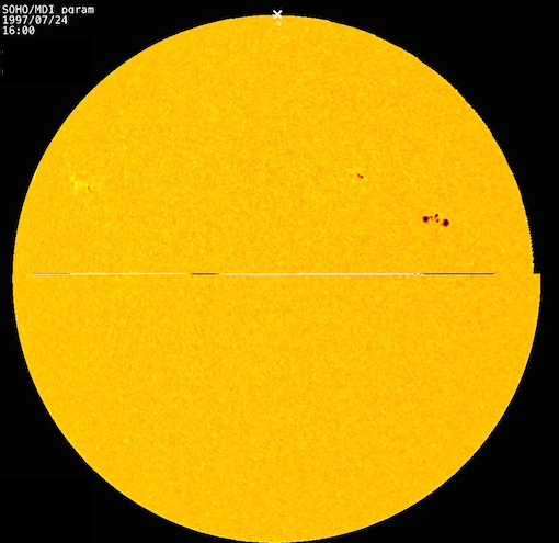
Other, rarely seen, missing-data interactions can produce unusual patterns of known vs. unknown values. We describe one below to illustrate how missing values interact with the rotate-and-merge approach. Below is a photogram interpolated from a later image that is complete, and an earlier one having its northern hemisphere missing. Thus, the southern hemisphere of the result is complete, but the west limb of the northern hemisphere has missing values. Unrelatedly, the erroneous line of values near the equator is an artifact at the edge of the missing data of the earlier image. We emphasize: this is rare.

Metadata

Most metadata names are the same as for the ordinary flattened 96-minute intensitygrams from mdi.fd_Ic_flat. The T_REC, T_OBS, and WCS are taken from the MDI magnetogram. Some quantities from the original intensitygrams are propagated forward into the interpolated intensitygram.

The following parameters internal to the interpolation process are also recorded:

QUALITY is the most important; it comes from the logical OR of the two constituent photograms, with the modifications mentioned above regarding time gap. (Note that the bits we introduce to capture the time gap, located at 0x70000, are not used by the constituent photograms.) Besides QUALITY, the most useful are IIXTCRIT, the weighted overall time gap, and IIP1_DT, IIP2_DT, the time-to-prior and time-to-next. Also of interest are the T_REC and T_OBS of the two source images.

Finally, there are segments PDATA1 and PDATA2 which are links to the earlier and later bracketing images.

Design Considerations

Effect of data gaps: There are about 72100 valid records in the series. About 1200 of these (1.6%) use trivial interpolation, and thus, in effect, contain no useful data. About 400 of these were during the very first months of the mission, and about 400 more were caused by various observing conditions in 2004. About 1500 further records (2.0%) had a "warning" level of IIXTCRIT, which is generally not problematic. About 250 were in 1996, and 400 during 2004. So in total, about 3.6% of data records had issues worth noting.

Differential rotation law: We tested other differential rotation laws besides the one used, including the one due to Snodgrass (1983). The results were not definitively better (judging using sunspots as tracers, across temporal gaps of around the maximum of 36 hours) than the law eventually used. As noted above, the differences among differential rotation laws result in at most a 1 pixel difference over 9 hours, which is not enough reason to definitively prefer one to the other in this application. Our conclusion is that the dominant effect on region coherence is gross morphology changes over time scales of 1–2 days, not alternate laws for differential rotation.

Perspective geometry: The rotation algorithm we used takes into account perspective effects due to the observer being at a finite distance from the Sun. As noted by Thompson (Astron. Astrophys. 515, A59, 2010), ignoring perspective causes a 2-arcsec (1 MDI pixel) error at around 0.7 solar radii. Additionally, because regions move tens of pixels along lines of constant latitude, computing correct latitude is important. A good criterion for correctness is to examine images with a small unipolar sunspot transiting the disk. If significant motion-prediction errors are made, the sunspot will jump or appear with a nearby ghost. We saw that using an observer-at-infinity model produced noticeable errors in some regions.

Linear weighting: In earlier work (TPM2000), we used a "switch" to combine rotated images into a single image. This switch chose, for each pixel, one image or the other to take data from, and corresponds to thresholding the weight w(i,j) described above. The present data product performs the merge via a linear combination (nonnegative weights, summing to one) of the two images. Of course, this causes a more smooth transition from one time to another. The practical benefit is that morphology changes (which appear to be the dominant source of error under normal comnditions) can be seen earlier, when the weight starts to deviate appreciably from zero or one, rather than at the midpoint where the thresholded value of w(i,j) jumps from 0 to 1 or vice versa.

Including dilation as a quality measure: Previously, we had only considered time difference in combining images: if δ₁ < δ₂, we would take the P₁' pixel if it was available, otherwise, we would fall back to P₂' (TPM2000). This produced noticeable artifacts as the last couple of columns of pixels at the east limb of P₁' was stretched over a large area in the resulting merged image. These artifacts prompted inclusion of dilation as well as time difference when combining the two images, and the improvement was quite evident.

No one-sided interpolation: Broadly speaking, we have attempted to either produce a full-disk interpolated image, or no image at all. Other approaches are possible: if only one bracketing photogram is found (the other being too distant in time), one could apply the rotation rule to the nearby image and allow all other pixels to be undefined. Such an approach would be helpful for some purposes, but because our goal is to perform region identification and full-disk tracking from these images, we did not want to produce artifacts like cut-off active regions. We did not feel the complexity of having some regions only partially present would be worth the small (less than 1.6%, see above) gain in coverage around the edges of the large data gaps in 1996 and 2004.

Conclusion and Usage

We described an MDI data series, mdi.fd_Ic_interp, that contains full-disk flattened intensitygrams that are in 1:1 correspondence with the MDI 96-minute cadence line-of-sight magnetograms in mdi.fd_M_96m_lev182. The two series share the same T_REC and T_OBS, and share all WCS parameters such as disk center, p-angle, and radius. This means that their data segments are aligned pixel-by-pixel, simplifying some analysis.

This intensitygram series is computed by finding bracketing MDI intensitygrams (from mdi.fd_Ic_flat, a 6-hour cadence series), rotating them forward and backward in time according to a differential rotation law, and projecting them into the LOS magnetogram coordinate frame. Care has been taken to account for geometric effects like perspective, foreshortening at the limb, and differential rotation.

The series can be used in a way similar to the intensitygrams in mdi.fd_Ic_flat. The main additional figure of merit for quality is the time gap over which interpolation is done, W. Two bits in the QUALITY keyword are provided for this. If QUALITY & 0x40000 (262144 decimal) is set (1.6% of images), then W > 36 hours and the image is just a placeholder and should not be used: it is in fact created as a disk of all ones. Thus, this bit must be checked. If QUALITY & 0x10000 (65536 decimal) is set (a further 2.0% of images), then W > 18 hours and the image is of lower quality, but still usable for most purposes. The numerical time gap W and other information related to the before and after source images are stored in metadata.